中小学教师“中部凹陷”问题

各省中小学教师工资水平的比较

各省中小学教师工资的差异在哪？现有统计数据中没有直接的数据。但统计数据中有各省各学段人员经费的总支出，而人员经费支出即是用于教师工资及福利的支出，该数值除以各省各段专任教师的数量，即可以在一定程度上反映各省中小学教师的工资水平。接下来我将以各省小学的人员经费数据和小学教师数量为例。

# setup
library(tidyverse)
library(rio)     
library(sf)
library(sjmisc)        # rec()
library(RColorBrewer)
library(here)
library(janitor)

# 各省教育财政支出数据导入与处理

## 1999-2006年数据
pexpend_06 <- import(here("files/middle_zone/expend_teacher.xlsx"), which = 1) %>%
  mutate(across(c(year:outlay_self), as.numeric))
## 2007-2019年的数据
pexpend_19 <- import(here("files/middle_zone/expend_teacher.xlsx"), which = 2) %>%
  mutate(across(c(year:outlay), as.numeric)) 

# 1999-2019年各省教师数据导入与处理
pteacher <- import(here("files/middle_zone/expend_teacher.xlsx"), which = 3) %>%
  mutate(across(c(year, teacher), as.numeric))

## 数据预处理
data_0719 <- pexpend_19 %>%
  select(province, year, sum_person) %>%
  left_join(pteacher, by = c("province", "year")) %>%
  drop_na(teacher) %>%
  mutate(salary = sum_person * 1000 / teacher)

data_9906 <- pexpend_06 %>%
  select(province, year, sum_person) %>%
  left_join(pteacher, by = c("province", "year")) %>%
  drop_na(teacher) %>%
  mutate(salary = sum_person * 1000 / teacher)

## 1999－2006，2007－2019年数据合并
salary_total <- bind_rows(data_9906, data_0719)

# 地图数据导入与处理
china <- st_read(here("files/middle_zone/china_shp"),quiet = TRUE)
china$NAME <- rec(china$NAME, rec="北京市=北京;天津市=天津; else=copy")

# 合并地图与教师工资数据
sh_salary <- china %>%
  right_join(salary_total,by=c("NAME"="province")) %>% 
  group_by(year) %>% 
  mutate(salary_d=findInterval(salary,quantile(salary,prob=0:4/4))) %>% 
  mutate(salary_dc=as.character(salary_d))

2019年各省小学教师工资水平分布情况

下图@fig-plot1 图 1 呈现的是2019年各省小学教师工资水平的空间分布情况，如图所示，可以发现一个重要事实：小学教师工资水平较低的省份主要是中部省份，而经济发展水平较低的省，比如西藏、青海，小学教师工资水平也中部河南江西要高。

ggplot() +
  geom_sf(data = china, size = 0.02) +
  geom_sf(
    data = filter(sh_salary, year == 2019),
    aes(fill = salary_dc), 
    size = 0.02, show.legend = F
  ) +
  scale_fill_brewer() +
  theme_void()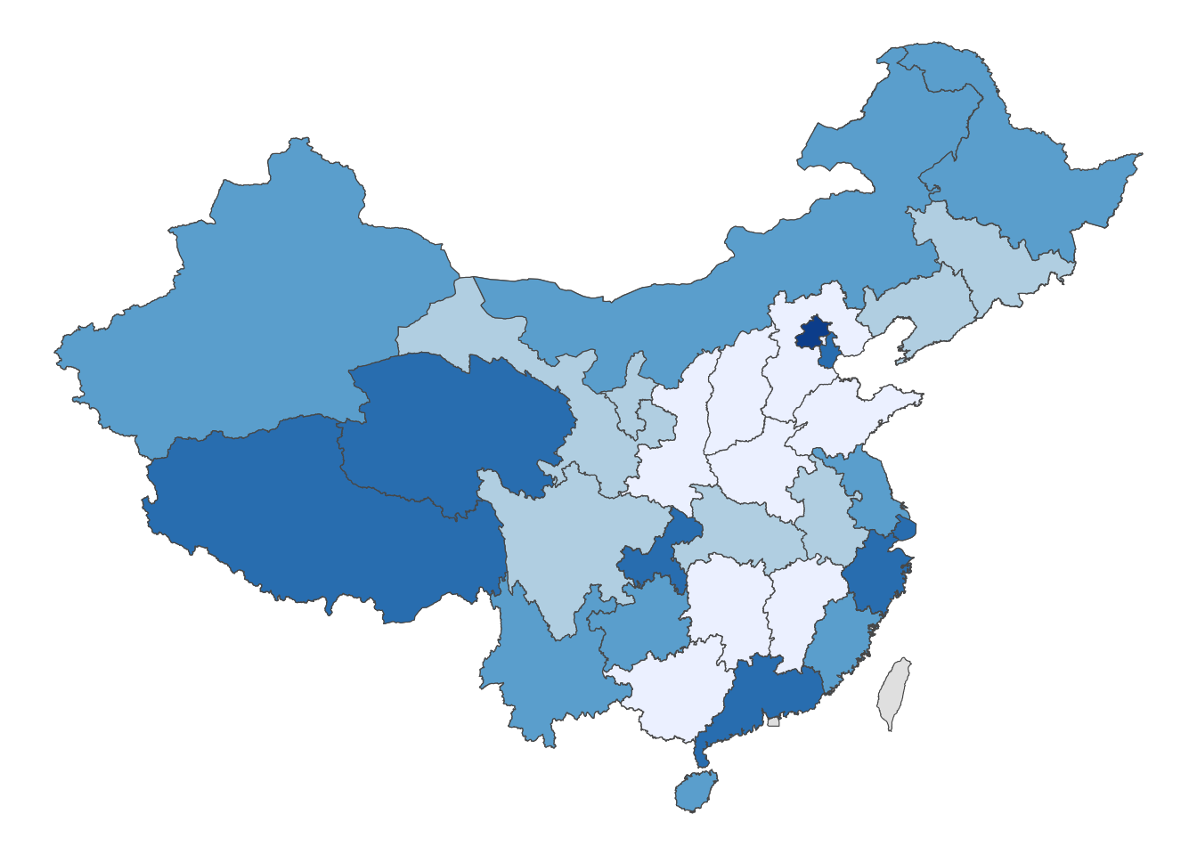

图 1: 2019年各省小学教师工资水平分布图

历年各省小学教师工资水平分布情况

上图只能反映2019年的状况，那么从历史角度来看是怎样的呢？下图 @fig-plot2 图 2 是1999至2019年各省小学教师工资水平的分布图，可以发现2019年各省小学教师工资水平的分布并不是一个截面的状态，而是一个长期现象。

ggplot() +
  geom_sf(data = china,size=0.02)+
  geom_sf(data=sh_salary,aes(fill=salary_dc),
          size=0.02,show.legend = F)+
  scale_fill_brewer()+
  theme_void() +
  facet_wrap(~year,ncol = 5)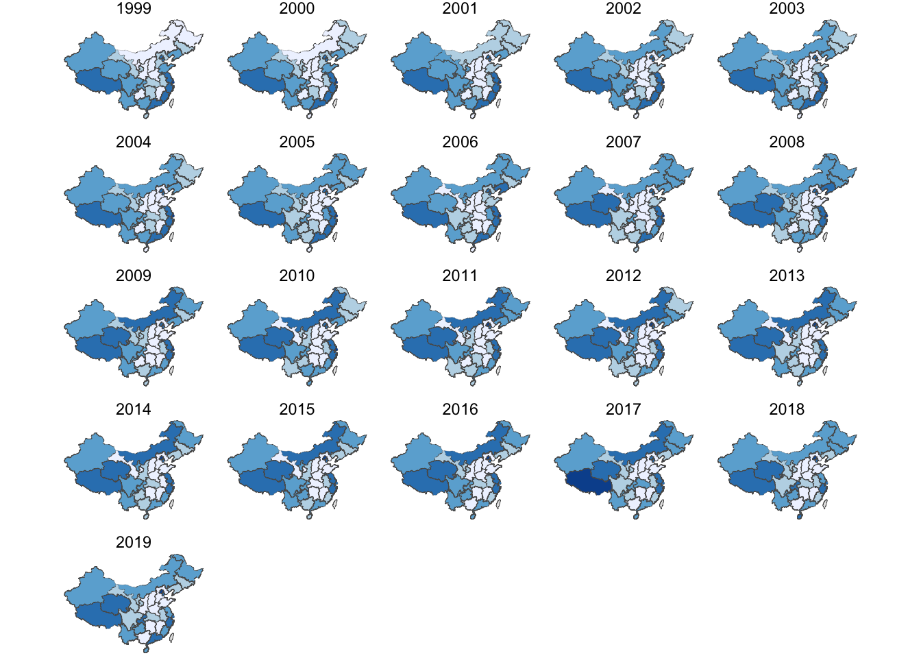

图 2: 1999-2019年各省小学教师工资水平分布图

中部凹陷为什么存在

首先想到的可能与各省的经济水平有关，下面来看一下各省人均GDP的分布。省级财政经费还有中央转移支付，我们也将看看中央转移支付占比与人均转移支付的问题。首先导入数据，数据主要是各省的GDP数据和财政收入与中央政府转移支付的数据。

#导入数据
##2011-2020年各省gdp数量
higher <- import(here("files/middle_zone/higheredu_gdp.xlsx"))
gdp <- higher %>% 
  select(province, starts_with("gdp")) %>% 
  drop_na(province) %>% 
  rename(name=province) %>% 
  pivot_longer(starts_with("gdp"),names_to="year", values_to = "gdp") %>% 
  mutate(year=parse_number(year))

##转移支付数据
transfer <- import(here("files/middle_zone/province_transfer.xlsx")) %>% 
  clean_names() %>% 
  mutate(total=str_detect(item,"Transfer")) %>% 
  pivot_longer(starts_with("x"),names_to = "year",values_to="revenue") %>% 
  mutate(total=as.factor(total)) %>% 
  select(province, year, total, revenue) %>% 
  pivot_wider(names_from = total, values_from = revenue) %>% 
  mutate(year=parse_number(year)) %>% 
  rename(total=`FALSE`,transfer=`TRUE`)

##1999-2019年各省财政收入、转移支付收入
transfer5 <- transfer %>% 
  filter(year>1998 & year<2020) %>% 
  mutate(ratio=transfer/total)

#各省人口数据(1949－2019)
popluation <- import(here("files/middle_zone/population.xlsx")) %>% 
  clean_names() %>% 
  mutate(type=str_detect(population,"城镇|乡村")) %>%    # 选择各省总人口数据
  filter(type==FALSE) %>% 
  mutate(name=str_sub(population,5)) %>% 　　            # 中文省名
  pivot_longer(starts_with("x"),
               names_to = "year",values_to="pop") %>% 
  mutate(year=parse_number(year)) %>% 
  select(name, province, year, pop)

##1999-2020各省人口数据
pop <- popluation %>% 
  filter(year>1998 & year<2020)

##合并人口与转移支付数据
trans_pop <- pop %>% 
  left_join(transfer5, by=c("province","year")) %>% 
  mutate(transfer_per=transfer/pop)

#区域指示数据
region <- import(here("files/middle_zone/china_zone.xlsx")) %>% 
  select(name,region)

#多个数据合并
data_triple <- salary_total %>% 
  rename(name=province) %>% 
  left_join(trans_pop,by=c("name","year")) %>% 
  left_join(gdp,by=c("name", "year")) %>% 
  left_join(region,by="name")

查看教师工资水平、人均GDP、转移支付占比之间的关系

下图 图 3 展示的是2019年各省小学教师工资水平的排序图，小学教师工资水平较低的省份依次是河南、河北、江西、山西、广西、陕西。水平较高的省份主要是北京、上海、西藏、天津、青海。图B和C，可以看出各省GDP与中央政府财政转移支付之间的互补关系。

theme_set(theme_bw(base_family = "KaiTi"))
plot_trans <- data_triple %>%
  filter(year == 2019) %>%
  ggplot() +
  geom_col(aes(y = fct_reorder(name, salary), x = ratio))+
  labs(y=NULL)

plot_gdp <- data_triple %>%
  filter(year == 2019) %>%
  ggplot() +
  geom_col(aes(y = fct_reorder(name, salary), x = gdp))+
  labs(y=NULL)

plot_salary <- data_triple %>%
  filter(year == 2019) %>%
  ggplot() +
  geom_col(aes(y = fct_reorder(name, salary), fill = region, x = salary))+
  scale_fill_brewer()+
  labs(y=NULL)

# comparion
library(patchwork)
plot_salary+plot_trans + plot_gdp+plot_annotation(tag_levels = 'A')

图 3: 2019年各省小学教师工资水平、人均GDP、转移支付占排序图

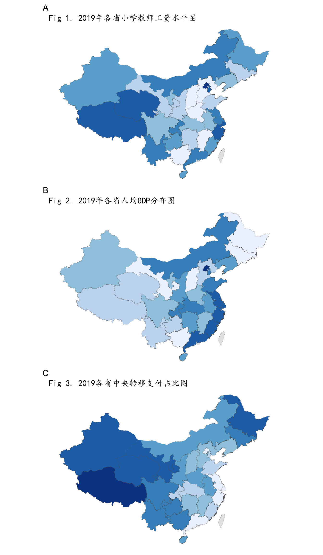
2019年各省教师工资水平、人均GDP、转移支付占比的空间分布图

我们以2019年各省小学教师工资水平为例，通过下图 图 4 可以发现：小学教师工资水平高的省份要么是本省人均GDP较高，要么是中央转移支付占比比较高。小学教师工资水平低的省份主要分布在中部地区，原因在于本省人均GDP不高，且中央转移支付的占比也不高。　

data2019 <- data_triple %>% 
  filter(year==2019)
sh_total <- china %>%
  right_join(data2019,by=c("NAME"="name")) %>% 
  mutate(salary_d=findInterval(salary,quantile(salary,prob=0:6/6)),
         ratio_d=findInterval(ratio,quantile(ratio,prob=0:6/6)),
         gdp_d=findInterval(gdp,quantile(gdp,prob=0:6/6)),
         ) %>% 
  mutate(salary_dc=as.character(salary_d),
         ratio_dc=as.character(ratio_d),
         gdp_dc=as.character(gdp_d))

plot1 <- ggplot() +
  geom_sf(data = china,size=0.02)+
  geom_sf(data=sh_total,aes(fill=salary_dc),size=0.02,show.legend = F)+
  scale_fill_brewer()+
  theme_void()+
  labs(title = "Fig 1. 2019年各省小学教师工资水平图")

plot2 <- ggplot() +
  geom_sf(data = china,size=0.02)+
  geom_sf(data=sh_total,aes(fill=gdp_dc),size=0.02,show.legend = F)+
  scale_fill_brewer()+
  theme_void()+
  labs(title = "Fig 2. 2019年各省人均GDP分布图")

plot3 <- ggplot() +
  geom_sf(data = china,size=0.02)+
  geom_sf(data=sh_total,aes(fill=ratio_dc),size=0.02,show.legend = F)+
  scale_fill_brewer()+
  theme_void()+
  labs(title = "Fig 3. 2019各省中央转移支付占比图")

(plot1/plot2/plot3)+plot_annotation(tag_levels = 'A')&
  theme(plot.title = element_text(family = "KaiTi"))

图 4: 2019年各省小学教师工资水平、人均GDP、转移支付占分布图